Welcome to CITYNEXUS PRO documentation!
CITYNEXUS PRO is an innovative urban digital twin application designed to assess the environmental, social, and economic impacts of changes in road networks, mobility systems, and urban space design. The platform also integrates climate-related hazards, including pluvial and surface-water flooding, to support climate-resilient urban planning.
Leveraging the DestinE platform, CITYNEXUS PRO evaluates baseline conditions of human mobility and urban dynamics by integrating key indicators such as air quality, dynamic population distribution, land-use allocation, service accessibility, flood exposure and the effectiveness of flood-defence measures, while enabling live, interactive what-if scenario analysis.
The platform is designed to provide policymakers a collaborative platform to experiment with various strategies and solutions, considering diverse factors and variables crucial for successful and sustainable urban interventions, thereby facilitating a coordinated approach to decision-making.
CITYNEXUS PRO Platform Overview
The CITYNEXUS PRO platform facilitates evidence-based decision-making at the municipal level by providing capabilities to evaluate a comprehensive set of Key Performance Indicators (KPIs) and by implementing an interactive system for assessing the impacts of infrastructural, mobility, and land-use changes on target KPIs through policy-relevant, user-defined what-if scenario simulations.
Currently, strategic decisions related to mobility and infrastructure interventions are often driven primarily by economic constraints, overlooking the complex, multi-dimensional impacts on neighbourhoods, communities, and urban systems. This limitation is further exacerbated by insufficient coordination and communication between districts within the same city or between neighbouring municipalities, making it difficult to assess the cumulative and cross-boundary effects of specific interventions.
To address these limitations, CITYNEXUS PRO offers policymakers a collaborative decision-support environment where alternative strategies and solutions can be explored systematically. The platform provides a comprehensive analytical framework that goes beyond cost-based assessments and explicitly accounts for user-defined priorities expressed through selected KPIs. These KPIs, identified in collaboration with end users, address multiple thematic areas, including:
Mobility Patterns: CITYNEXUS PRO provides detailed insights into commuting patterns, travel behaviour, traffic flows, congestion levels, peak traffic periods, and overall mobility dynamics, supporting transport planning and traffic management.
Air Quality: The platform evaluates ground-level concentrations of key atmospheric pollutants, including nitrogen dioxide (NO₂), sulfur dioxide (SO₂), carbon monoxide (CO), ozone (O₃), black carbon, and ultrafine particles.
Dynamic Population Distribution: CITYNEXUS PRO characterises human presence and movement patterns over time, enabling the analysis of population densities and temporal dynamics across different urban areas.
Service Accessibility: CITYNEXUS PRO evaluates the availability, accessibility, and equity of access to essential urban services, including transportation, healthcare, education, workplaces, commercial areas, and recreational facilities.
Flood Risk and Flood Defences: The platform assesses urban flood risk by analysing the spatial extent and severity of flooding and its impacts on infrastructure, accessibility, and mobility, while also enabling the evaluation of flood-defence measures and their effectiveness under extreme scenarios.
To support evidence-based decision-making at the municipal level, CITYNEXUS PRO operates at the local scale. To characterise seasonal patterns of human mobility and their relationships with the targeted KPIs, the platform is designed to operate on a quarterly temporal scale and to distinguish between typical weekdays and weekends. This approach enables the derivation of statistically robust baseline conditions for mobility and KPI characterisation, while also supporting the assessment of the impacts of what-if mobility and infrastructure interventions across different times of the year.
Four demonstration cities are currently available within the platform: Copenhagen (Denmark), Bologna (Italy), Seville (Spain), and Aarhus (Denmark). These cities were selected due to their alignment with the project’s focus on sustainable mobility, air quality improvement, climate adaptation, and urban innovation. In parallel, CITYNEXUS has been collecting manifestations of interest from additional cities wishing to be onboarded onto the platform and is currently working with the Bucharest Metropolitan Area and the City of Vitoria-Gasteiz to implement tailored deployments of the platform, reflecting their specific planning contexts and decision-making needs. Additional cities, public authorities, and user organisations are welcome to engage directly with the CITYNEXUS team to explore onboarding requirements, data needs, and implementation pathways for adopting the platform.
Data sources
CITYEXUS uses the following data sources:
High-Frequency Location-Based (HFLB) mobility data
Sentinel-5P TROPOMI Level-2 daily tropospheric vertical column densities for NO₂, SO₂, CO, and O₃
Copernicus Digital Elevation Model (DEM) of Europe at 10 m resolution
ECMWF ERA5 hourly meteorological estimates, including variables supporting hydrological and flood modelling
CORINE Land Cover (100 m resolution) from the Copernicus Land Monitoring Service
MERIT Hydro (~90 m resolution)
GEBCO 2023 Grid (~450 m resolution)
Copernicus Global Land Service products (~100 m resolution)
City-specific baselines and pre-defined scenarios
For each city available in CITYNEXUS PRO, the platform includes a baseline scenario that captures the current conditions, serving as a common reference against which all interventions are evaluated. This baseline reflects observed patterns of human mobility, land use, service accessibility, air quality, and climate-related exposure, ensuring consistency and comparability across analyses.
Building on this baseline, each city is equipped with a set of pre-defined, pre-loaded what-if scenarios that reflect policy measures, planning strategies, or intervention concepts that are locally relevant to that specific urban context. These scenarios are designed in close alignment with ongoing policy discussions or strategic objectives of each city, while remaining transferable and adaptable to other cities where relevant.
Copenhagen (Denmark)
The Copenhagen implementation includes scenarios addressing major mobility and land-use transformations aligned with the city’s climate-neutrality ambitions:
High-Speed Road Redesign, exploring the transformation of high-speed road segments into tunnels and the reallocation of surface space to residential uses, green areas, and recreational amenities.
Electric, Low-Emission Vehicles and Active Mobility Promotion, enabling users to customise the share of electric and low-emission vehicles and active mobility modes within the overall traffic fleet.
Road Speed Adjustment, allowing the assessment of speed-management policies across selected road segments or categories.
Seville (Spain)
The Seville implementation focuses on integrated measures targeting emissions reduction and modal shift:
Low Emission Zones (LEZ) Creation, enabling the designation of specific neighbourhoods or user-defined areas where motorised circulation is restricted or limited to specific vehicle classes
Eco-Mobility Campaign, combining Low Emission Zone creation with active mobility promotion to support the city’s objective of increasing cycling’s modal share while restricting high-emission vehicles in key urban areas.
Bologna (Italy)
The Bologna implementation reflects policies aimed at improving urban liveability and reducing traffic-related emissions:
Bologna Città 30, supporting the assessment of measures such as increased cycling shares and the introduction of 30 km/h speed limits in residential areas to enhance safety and reduce greenhouse gas emissions.
Creating custom what-if scenarios in CITYNEXUS PRO
In addition to these pre-defined scenarios, users are given the possibility to assess the effects of different types of interventions on the mobility patterns and all other targeted KPIs.
CITYNEXUS PRO also enables users to create custom what-if scenarios by parametrically configuring a set of urban, mobility, and climate-related variables. This allows users to design and test tailored intervention strategies aligned with specific planning questions or policy objectives.
Scenario definition
A scenario is defined by specifying the following parameters:
- Road segment properties, including:
Closing selected streets to motorised traffic
Converting surface streets into tunnels
Modifying maximum allowed speeds for individual road segments or road categories
- Hexagonal grid properties, including:
Defining or modifying land-use types within selected areas
Adding, removing, or reclassifying Points of Interest (POIs) that influence travel demand and accessibility
- Mobility fleet composition, including:
The percentage of bicycles in circulation
The percentage of electric vehicles relative to the total vehicle fleet
- Temporal context, including:
Type of day (weekday or weekend)
One or more 3-hour time slots, where three hours represent the minimum simulation timeframe
- Flooding:
Define precipitation characteristics, including onset, duration and intensity
Set values for river discharge and fluvial flow conditions
Set sea discharge and coastal water-level dynamics
Design flood-defence structures
What-if simulation outputs
Once a scenario is defined, CITYNEXUS PRO performs a what-if analysis for the selected parameters and time slots, generating simulations of the following outputs:
- Mobility statistics, including:
Fuel consumption
Average vehicle speed
Road occupancy levels
- Air and emission-related indicators:
Concentrations or emissions of five key pollutants: CO₂, CO, HC, NOₓ, and PMₓ
- Flood-related impacts, including:
Flood depth and spatial extent
All outputs are evaluated relative to the city baseline, enabling direct comparison between current conditions and alternative intervention scenarios
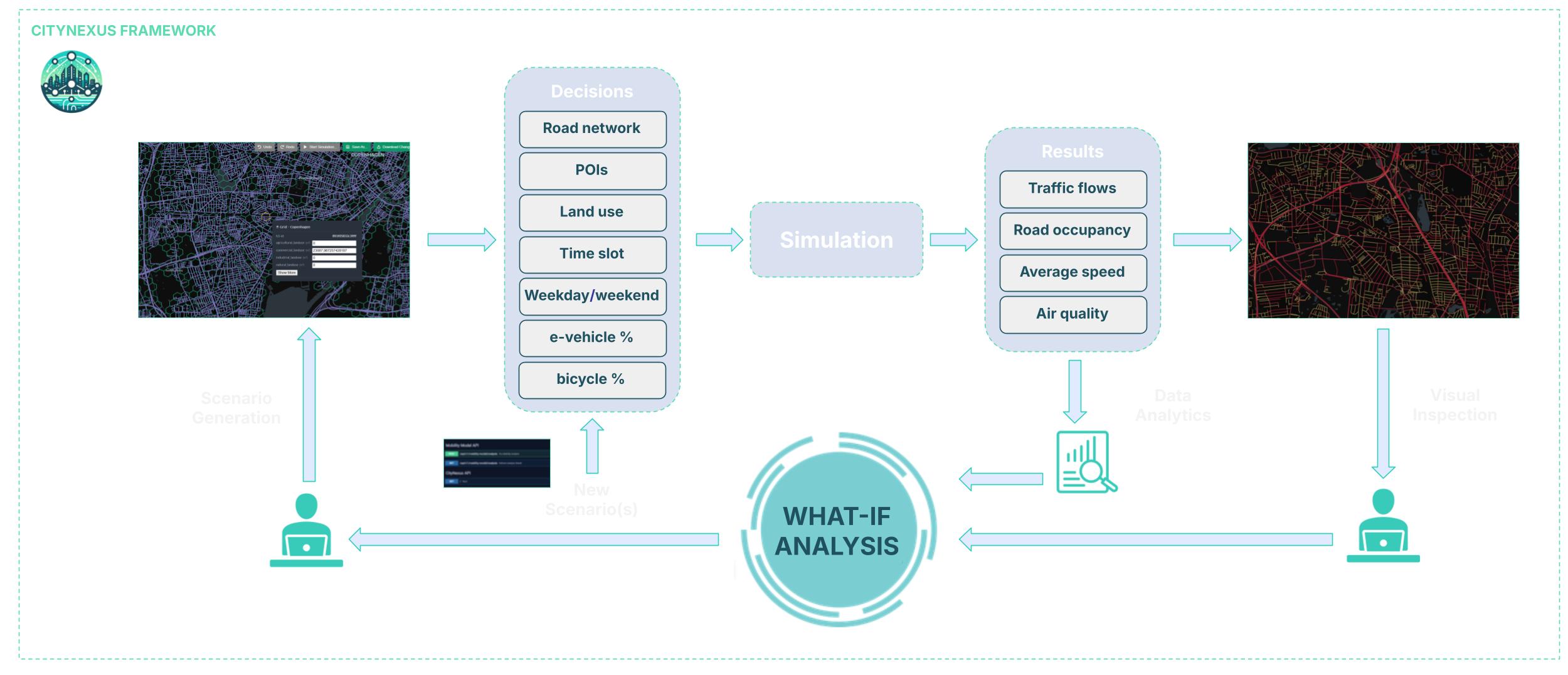
Figure 1 CITYNEXUS PRO framework
Figure 1 shows an overview of the CITYNEXUS PRO typical workflow. The user can create new scenarios by adjusting parameters such as the road network, land use, and vehicle types. Using these conditions, the system will then simulate traffic flow, congestion points, and air quality allowing the user to explore different outcomes and results that can be analyzed through interactive maps and animations. Some pre-defined scenarios are also available on the user workspace to explore the platform potentialities.