Eagle Service User Manual

Eagle visual workflow canvas in action — Eagle’s drag-and-drop workflow canvas: nodes are connected to build a geospatial AI pipeline that runs end-to-end without code.

1. Introduction to the Eagle Service 

1.1. Service Overview: The Earth Intelligence Studio 

Welcome to the Destination Earth Eagle service, the Earth Intelligence Studio. Eagle is a visual geospatial workflow platform that enables users to build, execute, and monitor AI-powered processing pipelines for Earth observation data – all without writing code.

The platform provides a drag-and-drop canvas where users connect processing nodes to create workflows for satellite imagery analysis, AI model inference, model fine-tuning, spectral analysis, zonal statistics, and result visualization.

1.2. Core Platform Capabilities 

Eagle is built around a visual workflow paradigm:

Visual Workflow Builder – An interactive canvas powered by React Flow where users design processing pipelines by dragging, connecting, and configuring nodes. Each node represents a discrete processing step (data source, preprocessing, AI model, output).
AI Model Ecosystem – Pretrained inference and fine-tuning pipelines for flood/water detection, burn scar detection, crop classification, solar farm detection (Satlas), rooftop solar panel detection, change detection, cloud detection (OmniCloudMask), field boundary detection (YOLO11), and text-prompted segmentation (SAM3).
Foundation-Model Backbones – Four interchangeable backbones (Prithvi, TerraMind, DOFA, Satlas) covering Sentinel-2, Landsat, and generic RGB sensors.
Integrated Data Access – Direct integration with the Copernicus Data Space for Sentinel-2 search and download. Support for GeoTIFF, Zarr, and NetCDF upload.
Analytical Tools – Interactive Spectral Analyzer, Zonal Statistics, Super Resolution (OpenSR), and GradCAM explainability.
Productivity Tools – LLM Workflow Assistant, Model Registry with versioning and comparison, Workflow Sharing via public links, and an Interactive Tour.

1.3. Understanding the Project-Based Workflow 

All work within Eagle is managed through a hierarchical structure:

Project – The top-level container for organising workflows, data, and results. Projects provide user-scoped isolation – each user sees only their own projects.
Workflow – A visual pipeline of connected nodes saved within a project. Workflows can be saved, loaded, shared, and re-executed.
Job – A single execution of a workflow. Jobs are tracked with per-node status, queued via the GPU-aware job scheduler, and recoverable after pod restarts.

This hierarchical model (User -> Project -> Workflow -> Job) is fundamental to the platform’s design.

2. Getting Started 

2.1. Authentication 

Eagle uses Destination Earth Keycloak SSO for authentication. Upon accessing the service URL, unauthenticated users see the landing page.

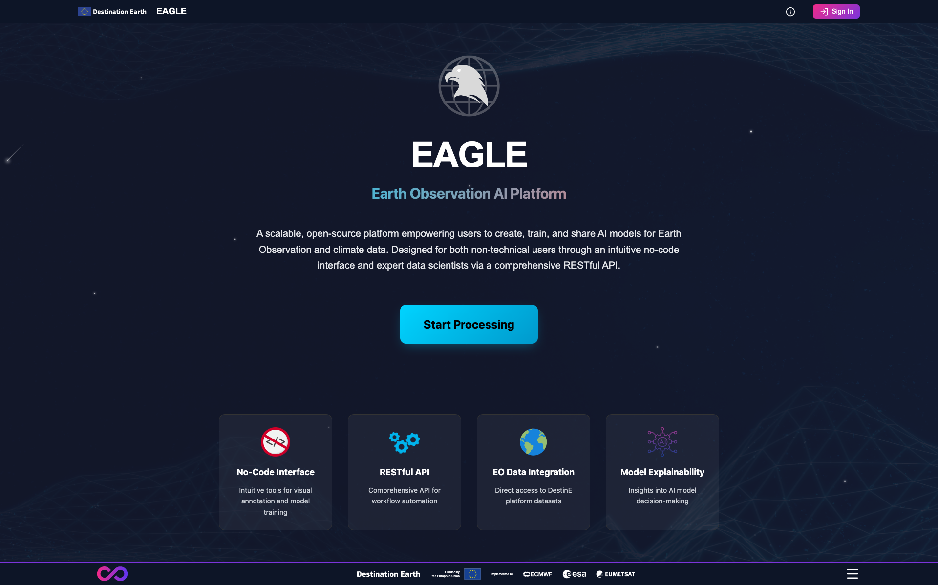
Eagle public landing page — Public landing page seen by unauthenticated visitors. Click **Start Processing** to be redirected to the Destination Earth IAM login.

Click Start Processing on the landing page.
You will be redirected to the Destination Earth authentication service.
Enter your credentials and complete any required verification steps.
After successful authentication, you are redirected back to the Eagle canvas.

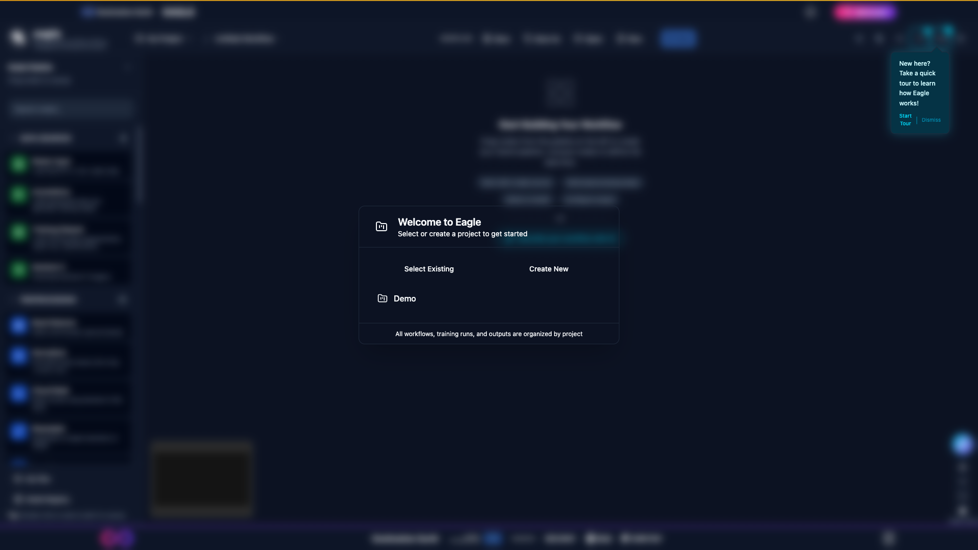
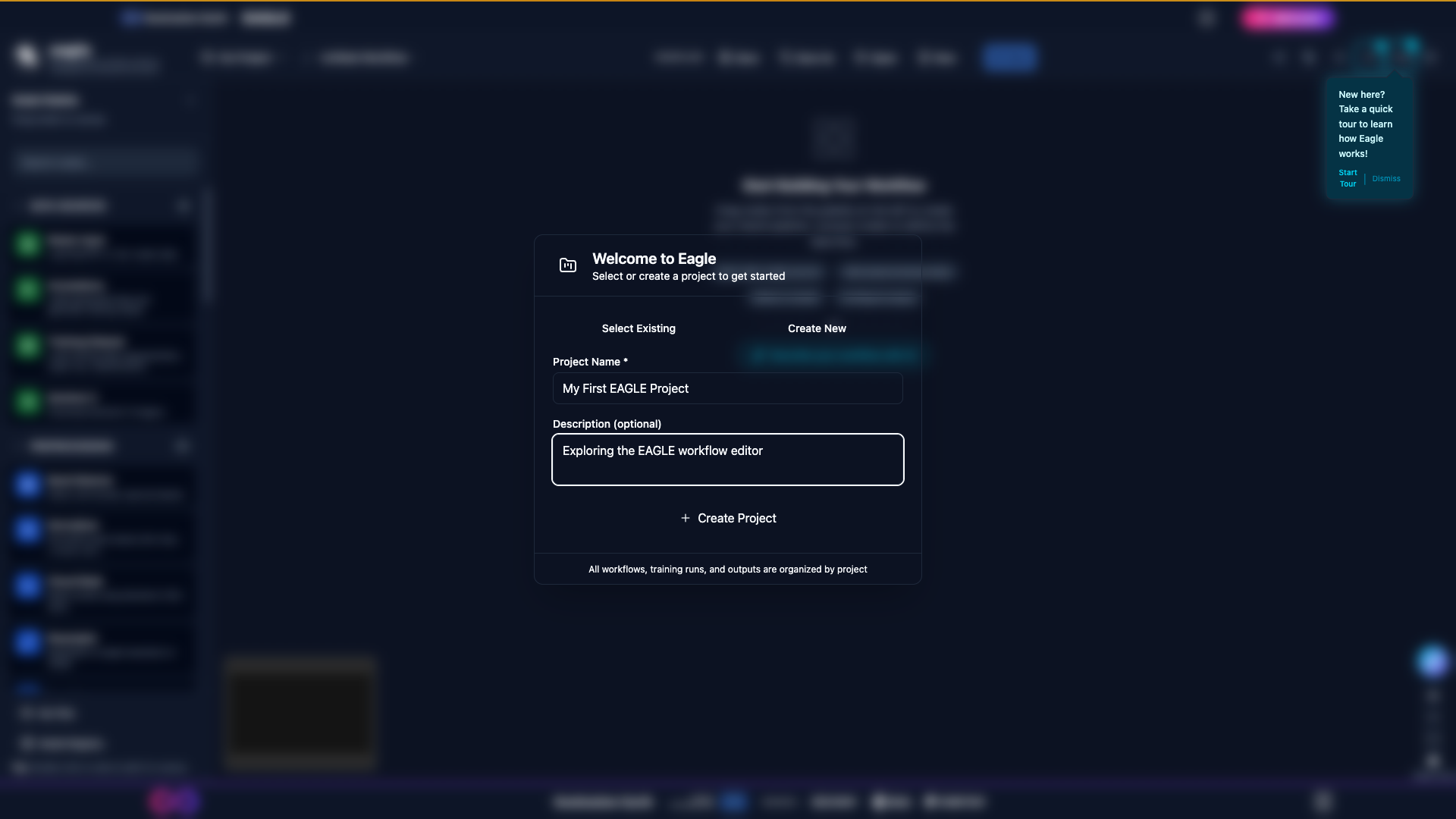
Welcome modal after first login — Welcome modal shown the first time you sign in, summarising the main capabilities of the Earth Intelligence Studio.

Note

Access tokens have a short validity and are automatically refreshed by the platform. Your session persists as long as the refresh token remains valid.

2.2. Creating Your First Project 

Projects are managed via the header project selector in the top navigation bar.

Click the project selector dropdown in the header.
Click Create New Project.
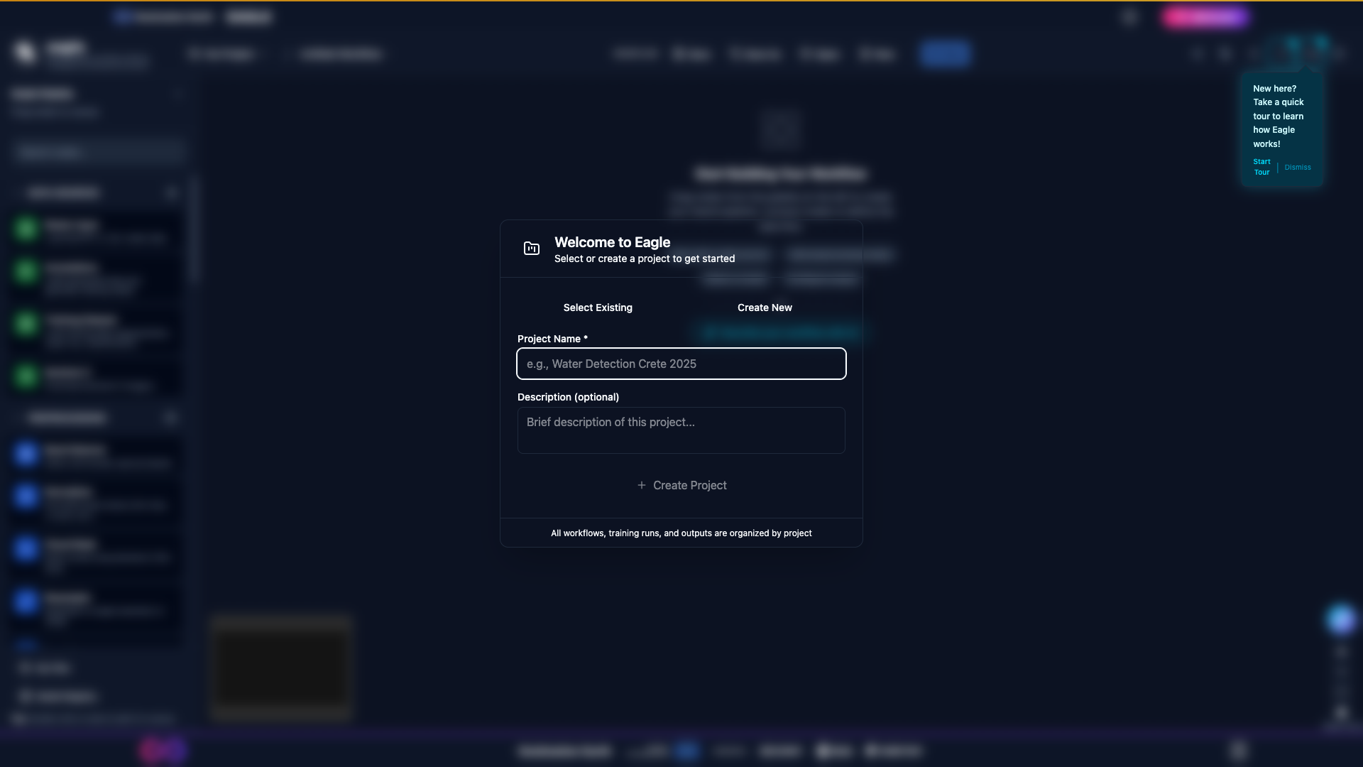
Enter a Project Name and optional Description.
Click Create to save the project.

Empty Create Project dialog — The **Create New Project** dialog before any input.

Create Project dialog with name and description filled in — The same dialog after filling in a name and description; click **Create** to confirm.

The new project is automatically selected as your active project. All workflows and jobs are associated with this project.

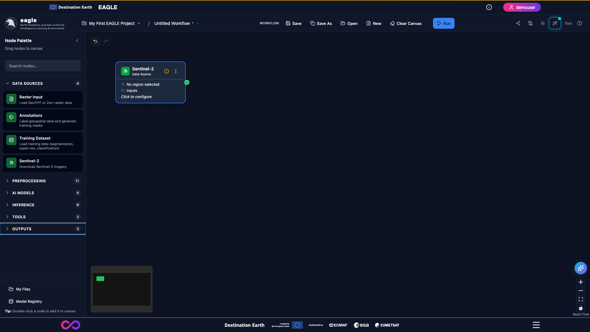
2.3. The Canvas Interface 

After authentication and project selection, you are presented with the main canvas interface:

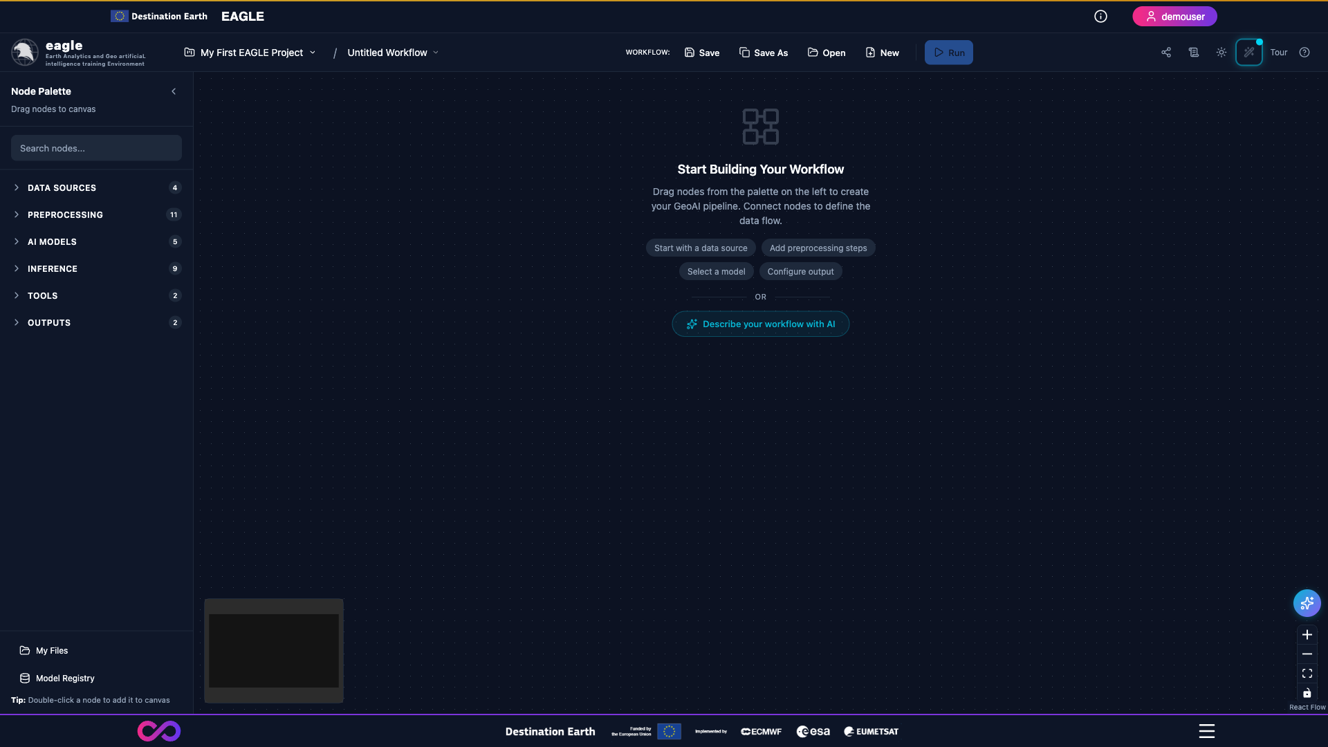
Empty Eagle canvas immediately after creating a project — The empty canvas shown after creating a project: header bar at the top, node palette on the left, and the React Flow workspace in the centre.

Header Bar – DESP branding, project selector, workflow name, Run button, Logs button (Operations Log), Share button, Tour button, and user controls.
Sidebar – Node palette organized by category with a search box at the top. Drag nodes from here onto the canvas, or double-click a node to place it at the canvas centre.
Canvas – The central React Flow workspace where you build workflows. Supports panning (click-and-drag), zooming (scroll wheel), and a Fit View button to reset zoom.
Help Guide – Open with F1 or ? for an in-app, searchable guide to every node, backbone, and feature, plus ready-to-run workflow templates.

Canvas with a transient toast notification after project creation — Toast notifications confirm important actions (project created, workflow saved, job submitted) and dismiss themselves automatically.

Eagle dashboard with multiple workflows in flight — A populated workspace: multiple nodes connected on the canvas with the operations panel and result previews open.

2.4. Keyboard Shortcuts 

Speed up your workflow with keyboard shortcuts:

Shortcut	Action
`Ctrl+S` / `Cmd+S`	Save workflow
`Ctrl+O` / `Cmd+O`	Open workflow
`F1` or `?`	Open the Help Guide
`T`	Toggle node tooltips
`Delete` / `Backspace`	Delete selected nodes or connections
`Click` a node	Select the node
`Ctrl+Click`	Multi-select nodes
Scroll wheel	Zoom in / out
Click + drag canvas	Pan view

3. Building Workflows 

3.1. Adding Nodes to the Canvas 

Two methods are available:

Drag and Drop – Click and drag a node from the sidebar onto the canvas, then release.
Double-Click – Double-click a node in the sidebar to add it at the canvas centre.

Use the search box at the top of the sidebar to filter nodes by name or description.

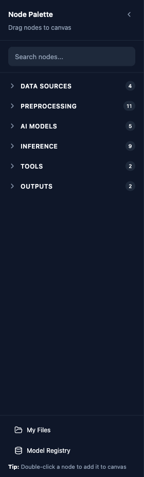
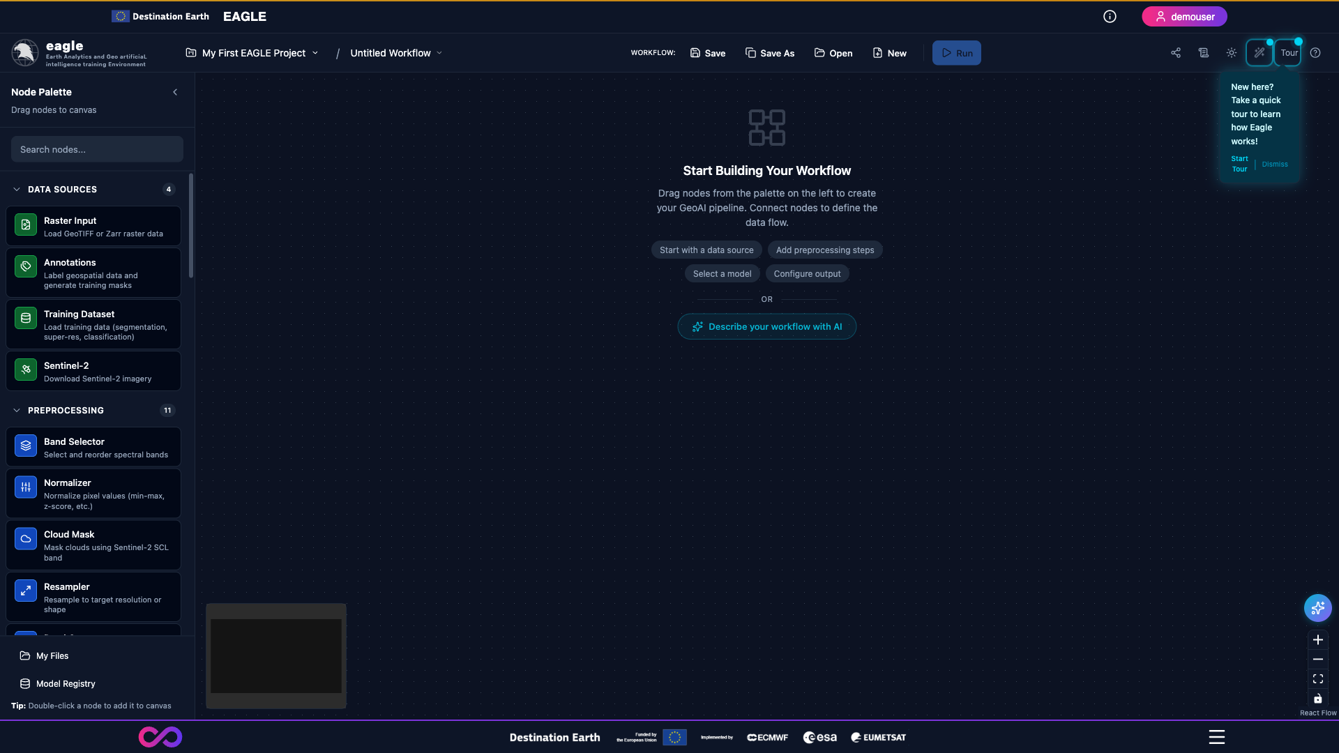
Node palette with all categories collapsed — The node palette with all categories collapsed. Click a category to expand it, or use the search box at the top to filter across all categories.

3.2. Node Categories 

Nodes are colour-coded by category:

Category	Colour	Nodes
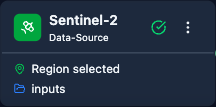
Data Sources	Green	Raster Input, Annotations, Training Dataset, Sentinel-2, Data Advisor (auto-run)
Preprocessing	Blue	Band Selector, Normalizer, Cloud Mask, Resampler, Band Converter, Band Stacker, Super Resolution, Save/Export, COG Converter, Tiler
Training	Purple	Flood/Water Training, Burn Scar Training, Crop Classification Training, Solar Farm Training (Satlas)
Inference	Cyan	Flood/Water Detection, Burn Scar Detection, Crop Classification, SAM3 Text, Change Detection, Field Boundary Detection, Cloud Detection (OmniCloudMask), Solar Panel Detection, Solar Farm Detection (Satlas)
Outputs	Yellow	Vectorize, Metrics

3.3. Connecting Nodes 

Nodes have input and output handles (coloured circles) that define data flow.

Hover over an output handle (right side, green circle) on a source node.
Click and drag to an input handle (left side, blue circle) on a destination node.
Release when the target handle highlights.

Connection rules enforce compatibility – incompatible nodes cannot be connected.

Category Compatibility:

From Category	Can Connect To
Data Source (green)	Preprocessing, Training, Inference, Output
Preprocessing (blue)	Preprocessing, Training, Inference, Output
Training (purple)	Inference, Output
Inference (cyan)	Output
Output (yellow)	Nothing (terminal)

Special Patterns:

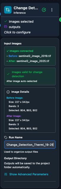
Change Detection – Two inputs: connect the earlier image to the before handle (top) and the later image to the after handle (bottom).
Band Stacker – Accepts multiple images on the same input handle; the stacked band order follows node-creation order.
Training -> Custom Inference – Run inference with a model you trained by enabling Use Custom Model on the inference node and selecting From Training Run.

To delete a connection, click it and press Delete or Backspace.

3.4. Configuring Nodes 

Click a node to open its configuration panel. Typical configuration includes:

Raster Input – File path to GeoTIFF, Zarr, or NetCDF. Supports File mode (single raster) and Folder (Batch) mode (run the same inference pipeline on each file in a folder).
Sentinel-2 – AOI (draw on map, enter coordinates, or Import AOI from a GeoJSON / zipped Shapefile), date range, cloud cover threshold, and band selection.
Training Dataset – Dataset type (Segmentation, Super-Resolution, Paired, Classification), folder paths, optional Zarr / NetCDF variable selection.
Inference / Training nodes – Backbone (Prithvi / TerraMind / DOFA / Satlas), DOFA sensor preset, tile size, batch size, device, GradCAM toggle.
Visualization – Colour maps, layer opacity, display options.

3.5. Workflow Templates 

Eagle ships with ready-to-run workflow templates available from the Help Guide’s Workflow Templates gallery:

Template	Difficulty	Description
Flood Detection Demo (Emilia-Romagna 2023)	Beginner	End-to-end demo with AOI, dates, bands and cloud cover pre-filled over the May 2023 Emilia-Romagna flood. Pick an output folder and click Run.
Flood / Water Detection	Beginner	Detect flooded areas and water bodies on Sentinel-2 imagery with the Prithvi pretrained model.
SAM3 Text Segmentation	Beginner	Text-prompted segmentation with SAM3.
Change Detection	Intermediate	SAM-based comparison of two images to detect landscape changes.
Fine-tuning with Raster Input	Intermediate	Train a custom model using a raster + Annotations workflow.
Fine-tuning with Training Dataset	Intermediate	Train a custom model using pre-existing images/masks folders.
Sentinel-2 Download & Export	Beginner	Download Sentinel-2 imagery and export it with band selection.
Sentinel-2 Download & Annotate	Beginner	Download Sentinel-2 imagery and prepare it for annotation / training.
Solar Farm Detection (Satlas)	Beginner	Detect utility-scale solar farms with the pretrained Satlas model.
Solar Farm Fine-tuning (Satlas)	Intermediate	Fine-tune the Satlas solar farm model on your own labelled data.

Click Workflow Templates in the Help Guide, pick a template, then customise parameters for your own AOI / dates / bands.

3.5.1. Preparing a Dataset for Fine-Tuning with Raster Input 

The Fine-tuning with Raster Input template trains a custom model from a user-provided raster plus an annotation project. To run the template you need:

A multi-band GeoTIFF uploaded via the File Browser. For the default Prithvi flood-detection backbone the expected channel order is B02, B03, B04, B8A, B11, B12 (six Sentinel-2 reflectance bands). TerraMind accepts the same six; DOFA adapts to whichever sensor preset you pick.
An annotation project created via the Sentinel-2 Annotation workflow or the Annotations panel, containing polygon labels over the same raster. For binary tasks (e.g. flood / not-flood) use two classes; the training node’s numClasses must match.
A recommended tile size of 224 x 224 pixels with 32 px overlap (matches the default tileSize / overlap used by the inference nodes so the fine-tuned checkpoint is drop-in compatible).

Starter dataset: the Sen1Floods11 hand-labelled subset (446 globally distributed 512 x 512 Sentinel-1/Sentinel-2 chips with water masks) at https://github.com/cloudtostreet/Sen1Floods11 is a small public dataset suitable for trying the workflow. Download one or more scenes, upload the Sentinel-2 GeoTIFF, convert the accompanying mask to polygons via the Sentinel-2 Annotation workflow, then run the template.

A recommended on-disk layout for organising your own datasets inside the project workspace is:

project-data/
├── rasters/
│   └── s2_my_aoi_2024-06.tif        # multi-band GeoTIFF
└── annotations/
    └── flood_labels.geojson          # polygon labels with class field

4. Node Reference 

4.1. Data Sources 

Raster Input – Load a raster from the project filesystem. Supports GeoTIFF, Zarr, NetCDF. Two modes:

File – Load a single raster. On load, the Data Advisor automatically analyses pixel quality (NaN %, nodata %, spatial coverage, constant bands, per-band statistics) and shows which training / inference tasks the data is compatible with.
Folder (Batch) – Load a folder of rasters and run the same inference pipeline on each file. Use for batch inference; for training use the Training Dataset node instead.

Annotations – Label geospatial data and generate training masks. Inputs: Image. Outputs: Masks. Configuration: project name, label definitions.

Training Dataset – Load pre-existing training data. Supports four dataset types:

Segmentation – Two folders (Images + Masks), files matched by basename.
Super-Resolution – Two folders (Low-res + High-res), matched by basename.
Paired – Two folders (Input + Target), general-purpose paired data.
Classification – One folder containing class subfolders; each subfolder name is the class label.

Drag & drop .zarr folders or .nc files is supported, including variable selection for both input and target stores. For folders with more than ~1000 files, use “click to browse” instead of drag & drop.

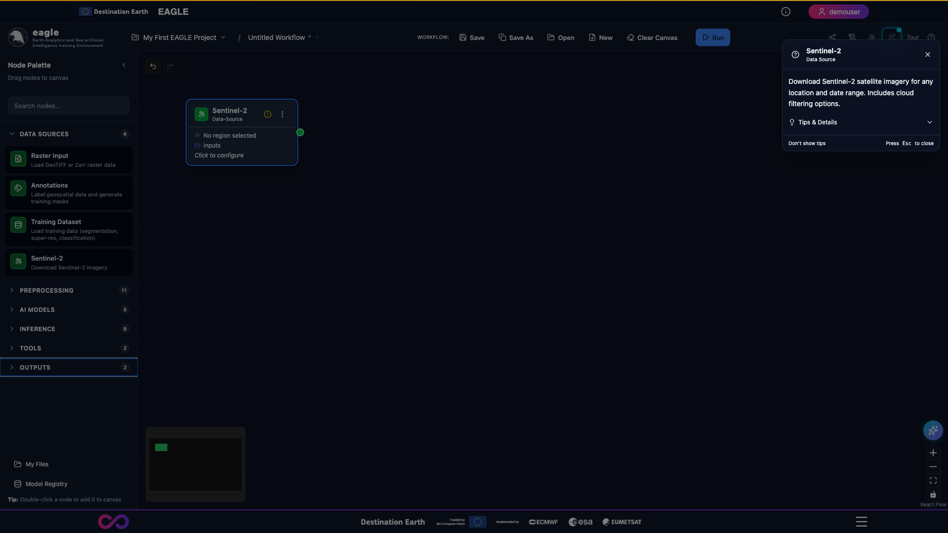
Sentinel-2 – Download Sentinel-2 imagery from ESA Copernicus. Configuration: AOI, date range, cloud coverage, band selection.

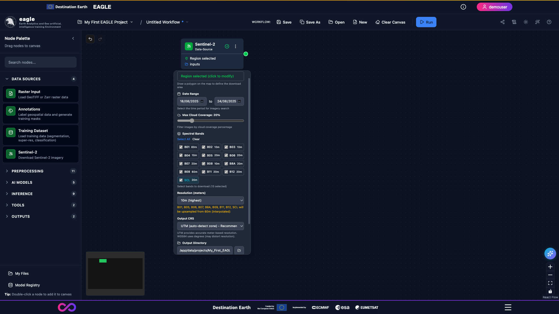
Sentinel-2 node with AOI, dates, cloud cover and bands configured — A fully configured Sentinel-2 node: AOI drawn on the map, date range set, cloud-cover threshold and band selection chosen.

Close-up of the Sentinel-2 node configuration panel showing the parameter inputs.

Scrolling through the Sentinel-2 node parameters — Scrolling through the Sentinel-2 node’s main parameters.

Walkthrough of all Sentinel-2 node options — Full walkthrough of the Sentinel-2 node options including AOI tools, date pickers, cloud-cover slider, and band selector.

Navigate by coordinates – enter Lat / Lon values in the map header to jump to a specific location.
Import AOI – click the green Import AOI button to load a polygon from a GeoJSON file (.geojson, .json) or a zipped Shapefile (.zip with a single layer). Multi-layer ZIPs are not supported.
The map shows country names, cities, and place labels for easy navigation.
After download completes, the Data Advisor automatically analyses the result.

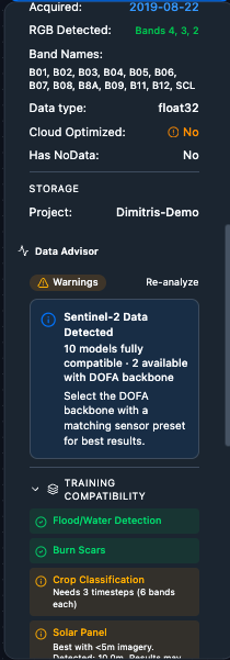
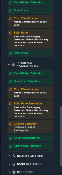
Data Advisor – Runs automatically whenever a Raster Input or Sentinel-2 download completes. Reports:

Quality Metrics – NaN %, nodata %, spatial coverage, constant bands, per-band statistics.
Training Compatibility – which training tasks your data is compatible with.
Inference Compatibility – which inference tasks your data can run.
Resource Estimates – file size, estimated tile count, GPU memory estimate.

Compatibility uses a three-colour system: green (fully compatible), amber (compatible with a note, e.g. “Needs 3 timesteps”), red (incompatible – missing required bands or insufficient band count).

4.2. Preprocessing 

Band Selector – Select and reorder spectral bands from a multi-band image. Supports band renaming and explicit band mapping when input names are generic (Band_1, Band_2, …).

Normalizer – Normalize pixel values. Methods: min-max, z-score, divide, percentile.

Cloud Mask – Mask clouds using the Sentinel-2 Scene Classification Layer (SCL). Configuration: SCL band index, classification values to mask. For sensors without an SCL band, use the Cloud Detection (OmniCloudMask) inference node instead.

Resampler – Resample imagery to a target resolution or shape. Configuration: target resolution, interpolation method.

Band Converter – Convert image bands for model compatibility. Configuration: target bands, conversion method.

Band Stacker – Stack multiple images into a multi-band composite. Accepts multiple inputs on the same handle (order = node-creation order). Used for multitemporal crop classification (3 timesteps x 6 bands = 18-band stack).

Super Resolution (OpenSR) – Enhance spatial detail of Sentinel-2 10 m imagery using the ESA OpenSR latent diffusion model. Inputs: RGB at 10 m (optionally plus NIR). Outputs: 4-band image at 2.5 m (4x upscaled). The output always has 4 bands (B02, B03, B04, B08) regardless of whether 3 or 4 input bands are provided; with only 3 RGB bands, the red channel is duplicated as a synthetic NIR before processing. Processing uses 128 x 128 tiles with overlap blending (no size limit) and runs on GPU when available.

Save / Export (terminal export step) – Save processed data to disk as GeoTIFF or Zarr. Configuration: output directory, filename, compression. Cannot connect to inference or training nodes.

COG Converter (terminal export step) – Convert raster to Cloud Optimized GeoTIFF with internal tiling and overview pyramids for fast web streaming. Configuration: block size, compression, overview levels. Cannot connect to inference or training nodes.

Tiler (terminal export step) – Split a large raster into tiles for training data preparation. Outputs: folder of tile files. Configuration: tile size, stride, edge handling. Cannot connect to inference or training nodes.

Note

Export steps (Save/Export, COG Converter, Tiler) write files to disk and are meant as final steps in a workflow. If you need to run inference, connect your data source (with optional preprocessing like Band Selector or Normalizer) directly to the inference node.

4.3. Training (AI Models)

All training nodes accept Images + Masks (from Annotations or Training Dataset) and output a Trained Model plus Metrics.

Flood / Water Detection Training – Backbones: Prithvi (6 bands), TerraMind (12 bands), DOFA (flexible via sensor preset).
Burn Scars Training – Same backbone options.
Crop Classification Training – Multitemporal input. Prithvi: 18 bands (6 x 3 timesteps); TerraMind: 36 bands (12 x 3); DOFA: flexible x 3 timesteps.
Solar Farm Training (Satlas) – Fine-tune the pretrained Satlas Swin-V2-B model. Required 9 bands: B04, B03, B02, B05, B06, B07, B08, B11, B12. Default 20 epochs, batch size 8. Segmentation head.

DOFA sensor presets (only shown when DOFA backbone is selected):

Sentinel-2 (6 bands) – default, same as Prithvi.
Sentinel-2 Full (12 bands) – all S2 L2A bands.
Landsat-8/9 (7 bands) – Landsat OLI bands.
RGB Only (3 bands) – any RGB imagery.

DOFA adapts its embeddings based on wavelength metadata, so it works with any sensor. Training and inference must use the same sensor preset.

Minimum training requirements: at least 10 training tiles. The train / validation split ensures at least 6 training and 2 validation samples. Use smaller tile sizes (128-256) if you need more tiles from limited annotations.

Important

Always connect a Metrics node after your training node. It provides real-time loss curves, best validation metrics (IoU, accuracy), early-stopping notifications, and epoch-by-epoch progress tracking.

4.4. Inference 

Flood / Water Detection – Pretrained Prithvi checkpoint (6 bands) or custom checkpoint with TerraMind / DOFA. Outputs a binary water-probability mask. GradCAM available.

Burn Scar Detection – Pretrained Prithvi checkpoint (6 bands) or custom TerraMind / DOFA. Binary burn-probability mask. GradCAM available.

Crop Classification – Multitemporal (3 timesteps). Pretrained Prithvi (18 bands) or custom TerraMind / DOFA. Per-class crop mask. GradCAM available – select the target class, run, and re-run with a different class to compare.

SAM3 Text – Text-prompt-based zero-shot segmentation. Inputs: any RGB or multispectral image + text prompt. Configuration: text prompt, confidence threshold, output options.

Change Detection – SAM-based comparison of two co-registered images. Two inputs via the before and after handles; band counts must match.

Field Boundary Detection – Delineate Anything (YOLO11-based). Auto-extracts RGB from Sentinel-2 (B04/B03/B02), runs inference tile-by-tile with overlap merging via union-find, outputs an instance mask, GeoJSON polygons, and a colour overlay. Optimal at ~10 m resolution; auto-upscales coarser imagery.

Cloud Detection (OmniCloudMask) – ML-based cloud and shadow detection. Auto-detects Red / Green / NIR from raster metadata (Sentinel-2 B04 / B03 / B08). Outputs a 4-class mask: clear (0), thick cloud (1), thin cloud (2), cloud shadow (3), plus a binary cloud-free mask, cloud-free image, and statistics. Supports Sentinel-2, Landsat 8/9, PlanetScope, Maxar at 10-50 m.

Solar Panel Detection – Mask R-CNN (geoai-py) instance segmentation for rooftop and ground-mounted panels on VHR imagery (0.3-2 m). Inputs: RGB. Outputs: instance masks + GeoJSON polygons.

Solar Farm Detection (Satlas) – Pretrained Satlas Swin-V2-B for utility-scale solar farms on Sentinel-2. Inputs: 9 bands (B04, B03, B02, B05, B06, B07, B08, B11, B12). Outputs: GeoJSON polygons. GradCAM available.

4.4.1. Change Detection: Step-by-Step 

This walkthrough shows how to build a Change Detection workflow that compares two co-registered rasters acquired at different dates and produces a binary change mask plus a side-by-side comparison view.

1. Build the workflow. From the node palette, drop two Raster Input nodes (one for the before image, one for the after image) and a Change Detection inference node onto the canvas.

Overview of a change-detection workflow on the canvas — The full Change Detection workflow: two Raster Input nodes feeding the *before* and *after* handles of a Change Detection node.

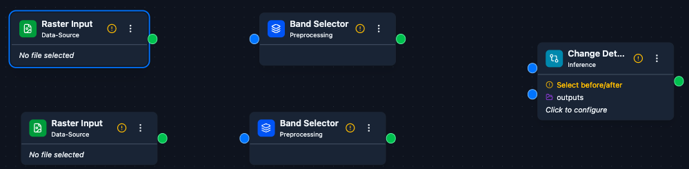
Three nodes placed on the canvas before connection — The three nodes added to the canvas, not yet connected.

2. Connect the nodes. Drag from the output handle of the first Raster Input to the before input of Change Detection (top), and from the second Raster Input to the after input (bottom).

Connecting a raster output to the before handle — Dragging a connection from a Raster Input output to the *before* handle of the Change Detection node.

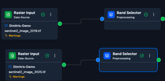
Workflow with both rasters connected to before and after — Both rasters wired up to the Change Detection node.

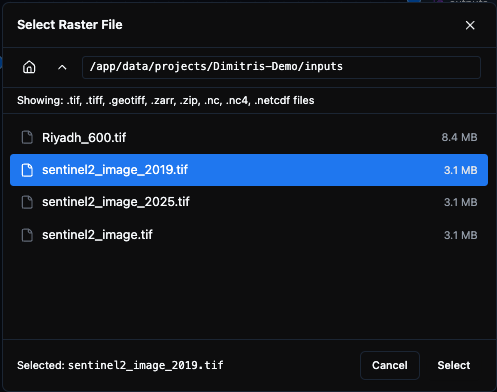
3. Configure each Raster Input. Click a Raster Input node to open its configuration panel and pick the file from the project filesystem.

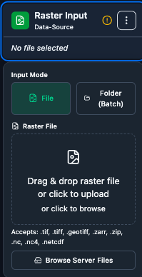
Empty Raster Input configuration panel — Raster Input configuration panel before selecting a file.

Selecting a node to open its configuration panel — Clicking a node selects it and opens the configuration panel on the right.

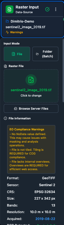
Raster Input panel after a file has been chosen — The panel updates with file details (path, size, CRS, band count) as soon as a raster is selected.

Raster Input panel for the before image — Configuration for the *before* raster.

Raster Input panel for the after image — Configuration for the *after* raster.

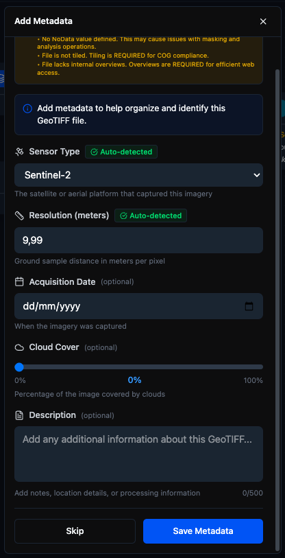
Raster metadata panel — The metadata panel surfaces band names, CRS, resolution, and the Data Advisor compatibility report.

Selecting which Raster Input feeds the before handle — Make sure the chronologically earlier raster is wired to the *before* handle – swapping the two will invert the change mask.

4. Preview the inputs. Click a Raster Input’s preview icon to view the image on the integrated map.

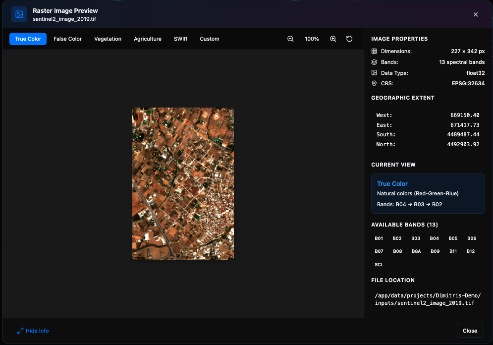
Preview of the 2019 before image — Preview of the *before* raster (2019 acquisition in this example).

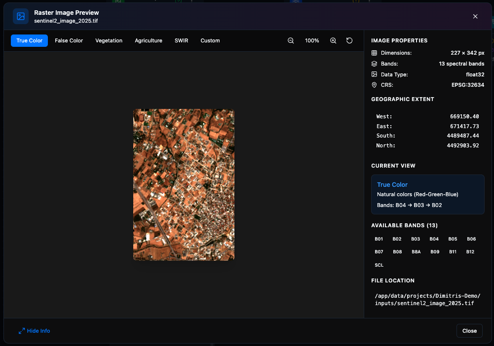
Preview of the 2025 after image — Preview of the *after* raster (2025 acquisition).

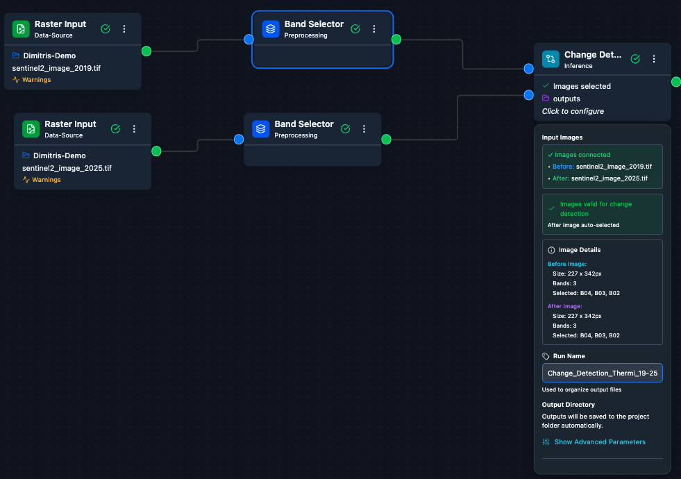
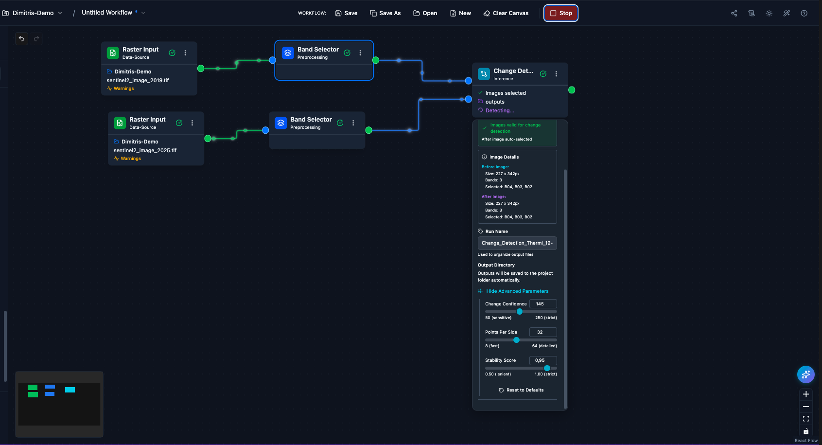
5. Tune the Change Detection node. Open the Change Detection configuration panel for band selection and optional advanced settings (threshold, simplification, post-processing).

Change Detection settings panel — Main Change Detection settings.

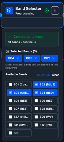
Band selector inside the Change Detection node — Band selector: pick the bands used to compute the change signal (band counts on the *before* and *after* inputs must match).

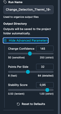
Advanced Change Detection options — Advanced options for fine-tuning the detection threshold and the post-processing of the binary mask.

6. Run the workflow. Save the workflow (Ctrl+S) and click Run in the header.

Click Run in the header to submit the job — Click **Run** to validate and submit the job to the GPU queue.

Workflow running with per-node progress — While the job is running, each node shows its own progress indicator.

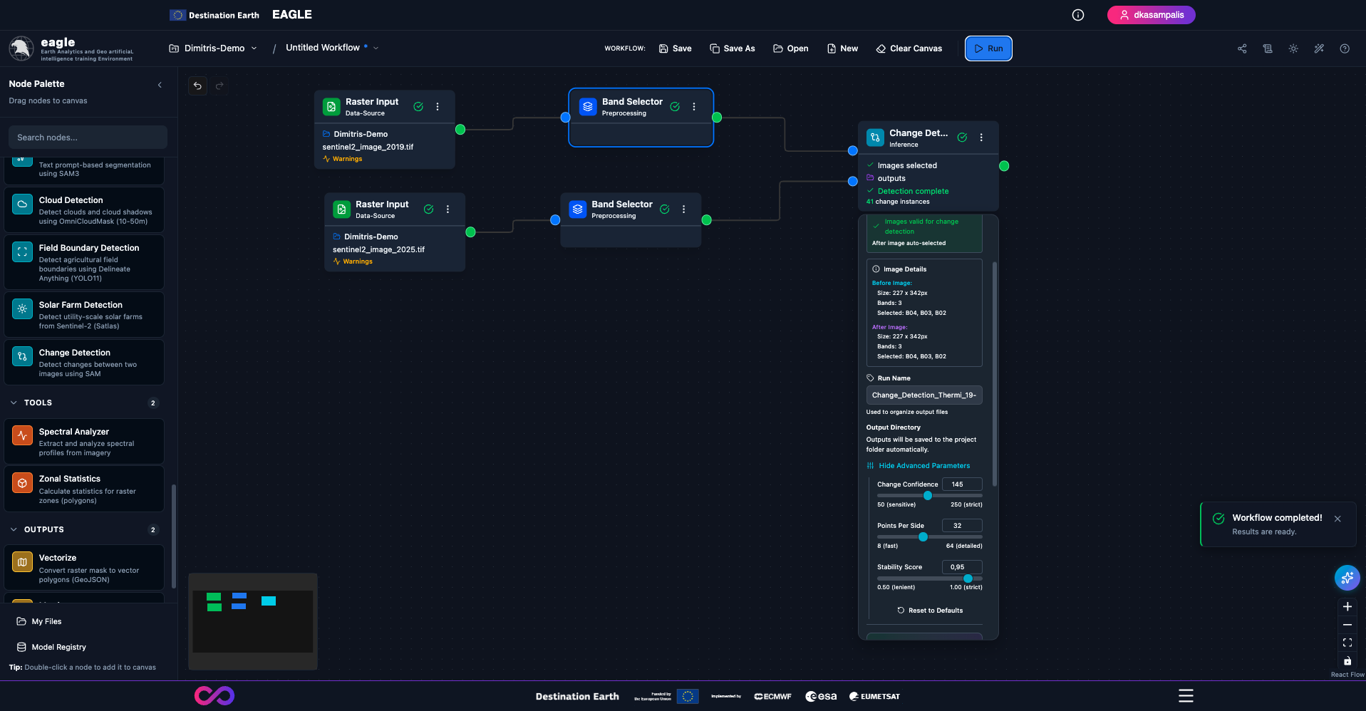
Workflow nodes marked completed — All nodes turn green once the job completes.

7. Inspect the results. Open the result previews and compare the two epochs side-by-side.

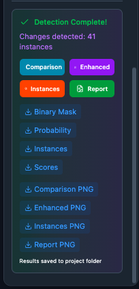
Change detection results map — Change-mask result rendered on the map; the legend explains the change classes.

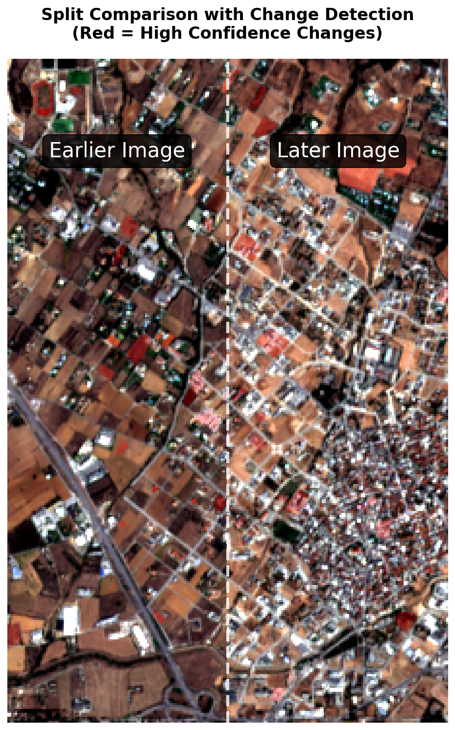
Split comparison view of the before and after images — The split-comparison view places the two rasters side-by-side with a draggable swipe so you can validate detected change visually.

4.4.2. Explainable AI (GradCAM)

All segmentation inference nodes support GradCAM – a visual heatmap showing which image regions most influenced the prediction.

Open the inference node’s configuration panel.
Toggle Enable Explainability (GradCAM) on.
For multi-class nodes (Crop Classification), select the Target Class from the dropdown.
Run the workflow – the GradCAM heatmap is saved alongside the prediction output as *_gradcam.tif.
After completion, click the XAI badge on the node to view the heatmap overlay. Red / warm regions indicate high model attention; blue / cool regions indicate low attention.

GradCAM explains one class at a time – change the target class and re-run to compare. Works with both pretrained and custom fine-tuned checkpoints. DOFA uses HiResCAM internally for higher-quality heatmaps.

4.5. Outputs 

Vectorize – Convert a raster mask to GeoJSON polygons. Configuration: output path, target class, simplify tolerance, minimum area.

Metrics – Display training progress and accuracy metrics. Inputs: Trained Model. Shows real-time loss curves (train + validation), best validation metrics (IoU, accuracy), early-stopping alerts, and epoch-by-epoch progress.

5. Foundation Models 

Eagle uses foundation models – large AI models pretrained on vast satellite imagery datasets – as the backbone for all training and inference tasks. Rather than training from scratch, fine-tune these backbones on your specific task, which requires far less data and time.

5.1. Overview 

Task	Backbones	Type	Pretrained	Input
Flood / Water Detection	Prithvi, TerraMind, DOFA	Segmentation	Prithvi only	Sentinel-2 (or any sensor via DOFA)
Burn Scar Detection	Prithvi, TerraMind, DOFA	Segmentation	Prithvi only	Sentinel-2 (or any sensor via DOFA)
Crop Classification	Prithvi, TerraMind, DOFA	Segmentation	Prithvi only	Multitemporal (3 timesteps)
Solar Farm Detection	Satlas Swin-V2-B	Segmentation	Yes	9-band Sentinel-2
Solar Panel Detection	Mask R-CNN (geoai-py)	Instance Segmentation	Yes	RGB aerial / VHR
Field Boundary Detection	YOLO11 (Delineate Anything)	Instance Segmentation	Yes	RGB (~10 m)
Cloud Detection	OmniCloudMask (geoai-py)	Segmentation	Yes	Red + Green + NIR (10-50 m)
Change Detection	SAM-based	Segmentation	Yes	Any (two images)
SAM3 Text Segmentation	SAM3	Prompt-based	Yes	Any RGB / multispectral

5.2. Backbone Architectures 

Prithvi EO v2 (IBM / NASA)

A 600 M-parameter Vision Transformer pretrained on 4.2 M global Sentinel-2 and Landsat time-series samples using Masked Autoencoder (MAE) self-supervised learning. Excels at capturing seasonal processes and land-surface dynamics.

Type: Vision Transformer (ViT-Large)
Input: 6 Sentinel-2 bands (B02, B03, B04, B8A, B11, B12)
Decoder: UperNet, UNet, FCN, or Linear (configurable)
Pretrained task checkpoints: Yes (flood, burn scar, crop)
GitHub: https://github.com/NASA-IMPACT/Prithvi-EO-2.0

TerraMind v1 (IBM / ESA)

The first any-to-any generative foundation model for Earth observation. Processes all 12 Sentinel-2 L2A bands simultaneously, capturing richer spectral information including Red Edge, Water Vapor, and Coastal Aerosol bands. Features “Thinking-in-Modalities” capability for cross-modal reasoning.

Type: Multi-modal Vision Transformer
Input: 12 Sentinel-2 L2A bands (B01-B09, B11, B12)
Pretrained task checkpoints: No (fine-tune required)
GitHub: https://github.com/IBM/terramind

DOFA Large (Dynamic One-For-All)

A wavelength-adaptive foundation model that works with any satellite sensor. Uses a Dynamic Weight Generator (neural hypernetwork) to create unique convolutional kernels per band based on its wavelength. Pretrained on five modalities: Sentinel-2, Sentinel-1 SAR, NAIP aerial, EnMAP hyperspectral, and Landsat.

Type: Vision Transformer (ViT-Large) with Dynamic Weight Generator
Input: Flexible – any number of bands, any sensor, via sensor preset (Sentinel-2 / Sentinel-2 Full / Landsat-8/9 / RGB)
Pretrained task checkpoints: No (fine-tune required)
GradCAM: HiResCAM for better explainability
GitHub: https://github.com/zhu-xlab/DOFA

Satlas Swin-V2-B (Allen AI)

A family of task-specific models trained on 302 million labels across global Sentinel-2 imagery. Uses a Swin Transformer V2-B backbone with Feature Pyramid Network (FPN) for multi-scale feature extraction and task-specific heads.

Type: Swin Transformer V2-B + FPN
Input: 9 Sentinel-2 bands or 3 RGB bands (task-dependent)
Heads: segmentation, point detection, regression
Pretrained task checkpoints: Yes (solar farm)
Website: https://satlas.allen.ai

5.3. Pre-trained Model Training Data 

The pre-trained checkpoints shipped with Eagle are fine-tuned on publicly released, peer-reviewed Earth observation datasets:

Task	Backbone	Training dataset
Burn Scar Detection	Prithvi-EO 2.0 (300M)	HLS Burn Scars – 804 HLS scenes (harmonised Landsat + Sentinel-2, 6 bands) with binary burn/no-burn masks. https://huggingface.co/datasets/ibm-nasa-geospatial/hls_burn_scars
Flood Detection	Prithvi-EO 2.0 / TerraMind / DOFA	Sen1Floods11 – 4,831 512x512 chips from 11 globally distributed flood events with hand-labelled water masks. https://github.com/cloudtostreet/Sen1Floods11
Multitemporal Crop Classification	Prithvi-EO 2.0 / TerraMind / DOFA	NASA HLS Multi-Temporal Crop Classification – CONUS 3-time-step HLS chips with 14 crop classes derived from USDA CDL. https://huggingface.co/datasets/ibm-nasa-geospatial/multi-temporal-crop-classification
Satlas Solar Farm	Satlas Swin-V2-B	SatlasPretrain – 856k Sentinel-2 / NAIP / Sentinel-1 image pairs labelled across 137 categories spanning infrastructure, land cover, and vegetation. https://satlas.allen.ai/

Note

The foundation backbones themselves are pre-trained by their upstream authors on much larger, unlabelled corpora (Prithvi-EO 2.0 on HLS v2; TerraMind on multi-modal Sentinel-1/2/DEM/land-cover data; DOFA on a diverse EO modality mix). The table above refers to the task-specific fine-tuning data used for the inference checkpoints exposed in Eagle, not the pre-training corpora of the backbones.

5.4. Choosing the Right Model 

Your Data / Priority	Recommended
Sentinel-2 (6 bands)	Prithvi backbone – pretrained checkpoints, proven performance
Sentinel-2 (all 12 bands)	TerraMind backbone – leverages full spectral range
Landsat-8/9	DOFA with Landsat-8/9 preset
Drone / Aerial RGB	DOFA with RGB preset
Sentinel-2 infrastructure mapping	Satlas models
Fastest setup (no training)	Prithvi or Satlas (pretrained)
Any object, no labels	SAM3 Text Segmentation (zero-shot)
Best accuracy on custom data	Fine-tune any backbone on your labelled data

General tips:

Always start with a pretrained checkpoint if available – it gives a strong baseline.
Fine-tuning typically needs 50-200 labelled tiles for good results.
Use GradCAM to verify the model is attending to sensible regions.
Training and inference must use the same backbone and band configuration.
Connect a Metrics node after training to monitor progress and early stopping.

6. Band Requirements 

6.1. Prithvi (6 bands)

Index	Band Name	Sentinel-2	Wavelength	Resolution
0	Blue	B02	490 nm	10 m
1	Green	B03	560 nm	10 m
2	Red	B04	665 nm	10 m
3	NIR	B8A	865 nm	20 m
4	SWIR1	B11	1610 nm	20 m
5	SWIR2	B12	2190 nm	20 m

If your raster has a different band order, use the Band Selector node to reorder bands before inference.

6.2. Satlas (9 bands, Solar Farm)

Satlas uses RGB-first order, which differs from Prithvi’s BGR order.

Index	Band Name	Sentinel-2	Wavelength	Resolution
0	Red	B04	665 nm	10 m
1	Green	B03	560 nm	10 m
2	Blue	B02	490 nm	10 m
3	Red Edge 1	B05	705 nm	20 m
4	Red Edge 2	B06	740 nm	20 m
5	Red Edge 3	B07	783 nm	20 m
6	NIR	B08	842 nm	10 m
7	SWIR1	B11	1610 nm	20 m
8	SWIR2	B12	2190 nm	20 m

6.3. DOFA Sensor Presets 

Preset	Bands	Band Names
Sentinel-2 (default)	6	B02, B03, B04, B8A, B11, B12
Sentinel-2 Full	12	B01-B09, B11, B12
Landsat-8/9	7	B1, B2, B3, B4, B5, B6, B7
RGB Only	3	B04, B03, B02

Training and inference must use the same sensor preset. For multitemporal tasks (Crop Classification), bands are repeated per timestep (e.g. Landsat = 7 x 3 = 21 bands).

6.4. Multitemporal Crop Classification 

Crop Classification requires multitemporal imagery. With the Prithvi backbone, 3 timesteps x 6 bands = 18 total bands, ordered as:

Bands 0-5: Timestep 1
Bands 6-11: Timestep 2
Bands 12-17: Timestep 3

Create the stack by loading three rasters (one per timestep) and connecting all three to a Band Stacker.

7. Executing and Monitoring Jobs 

7.1. Submitting a Workflow 

Save the workflow (Ctrl+S / Cmd+S).
Click Run in the header.
The workflow is validated (required parameters checked, connections verified).
If validation passes, the job is submitted to the GPU-aware job queue and a notification confirms the job ID.

7.2. The Operations Log 

Click the Logs button (scroll icon) in the header to open the Operations Log modal.

Operations are grouped by workflow execution. Expand a workflow to see all operations that ran during that execution.
Three categories are tracked: Preprocessing (band selection, normalization, cloud masking, resampling), Training (epochs, loss, IoU, accuracy), and Inference (detection coverage, pixel counts).
Click an operation to expand and see configuration parameters, result metrics, duration, and timestamps.
Use the tabs at the top to filter by category: All, Preprocessing, Training, Inference.

All operations are saved to the database and persist across server restarts – you can review past executions at any time.

7.3. Job Queue Management 

Eagle uses a GPU-aware FIFO job queue.

Jobs are processed in submission order.
GPU resources are allocated automatically based on availability (one job per GPU).
CPU-only tasks (vectorization, spectral analysis) bypass the GPU queue and run immediately.
If a pod restarts, running jobs are marked FAILED and pending jobs are re-enqueued automatically.

8. Working with Results 

8.1. Previewing Results 

After a job completes, results can be previewed directly on the canvas:

GeoTIFF outputs render as map layers with configurable colour maps.
Vector outputs (GeoJSON) render as interactive overlays.
Statistics are shown in metadata panels with charts and summary metrics.

The preview panel includes a Map View (with base maps and drawing tools), a Metadata Panel (raster metadata, band information, CRS), and a Timeline Player for temporal analyses.

8.2. Downloading Results 

Click the Download button on a result node or in the Operations Log.
Select the output format (GeoTIFF, GeoJSON, etc.).
The file is packaged and downloaded to your browser.

8.3. File Browser 

Click the File Browser button to navigate the project’s directory structure, view file metadata, preview GeoTIFFs, and manage uploads.

9. Advanced Features 

9.1. Zonal Statistics 

Compute aggregate raster statistics (min, max, mean, std, percentiles, etc.) for pixels within polygon zones drawn on an interactive map.

Workflow:

Raster Input → (optional preprocessing) → Zonal Statistics

Opening Zonal Statistics: connect a Zonal Statistics node to a raster and click Open Zonal Statistics on the node panel.

Drawing zones: three tools in the toolbar on the left of the map:

Polygon – click to add vertices, double-click to finish.
Rectangle – click and drag to draw.
Freehand – click once to start, move to trace, click again to finish.

Available statistics (17+): min, max, mean, median, sum, count (Basic); std, range, variance (Distribution); P10, P25, P50, P75, P90 (Percentiles); majority, minority, unique (Frequency). Default selection is 9 common statistics; customise via the Settings panel.

Results:

Results Table (top-right) – one row per zone with colour swatch, editable name, area in hectares, pixel count, and statistics columns. Sort by clicking column headers; toggle visibility with the eye icon.
Bar Chart (bottom-right) – grouped bars per zone, switchable statistic via dropdown.
Choropleth Map – zones colour-coded by the selected statistic using a purple gradient.
Multi-Band – Band dropdown in the header switches the visible band; table and chart update accordingly.

Import / Export:

Import – load existing zones from GeoJSON (Feature / FeatureCollection, Polygon / MultiPolygon).
Export – JSON (full metadata), CSV (spreadsheet-ready), or GeoJSON (zone polygons with statistics as feature properties, ready for QGIS / ArcGIS).

Zone area is computed using UTM projection for accuracy. Zones and statistics persist between sessions once saved.

9.2. Spectral Analysis 

Interactive spectral profile extraction and analysis from raster imagery.

Opening the Analyzer: on a Raster Input node, click the spectroscopy icon (Activity) to open the full-screen modal.

Sampling modes:

Single Point – click anywhere on the map to extract a spectral profile. Each click creates a new profile.
Area Selection – enable in Settings, choose Grid Spacing (20 / 30 / 50 / 100 px), then drag a rectangle on the map to extract profiles at regular grid intervals.
Kernel sizes: 1x1 (single pixel), 3x3 (9-pixel average), 5x5 (25-pixel average).

Chart: wavelength (nm) on X, reflectance on Y. Each line = one profile (colour-matched to map markers). Hover for exact values. Click legend to toggle visibility.

Library: select / rename (double-click) / delete / toggle visibility / clear all. Bulk export to JSON (with full metadata) or CSV (spreadsheet-ready).

Groups: organize profiles by category (e.g. Forest / Water / Urban). Create in Settings, assign profiles before sampling. Group members share a colour palette.

Reference Spectra: built-in library (vegetation, water, soil, urban materials, minerals) plus custom CSV / JSON / TXT import. Visible references appear as dashed lines on the chart.

Spectral Indices (vegetation / water / built-up): NDVI, SAVI, EVI (vegetation); NDWI, MNDWI (water); NDBI, BSI (built-up / bare soil). Requires NIR (B08 or B8A), Red (B04), Green (B03), and for some indices SWIR (B11, B12).

Statistics: Mean, Std, Min, Max, Median, P25, P75 computed across visible profiles. Chart overlay shows mean line with std envelope.

Multi-source: connect multiple Raster Input nodes for temporal / sensor / band-configuration comparison. Source dropdown switches between images; each source has a distinct colour palette.

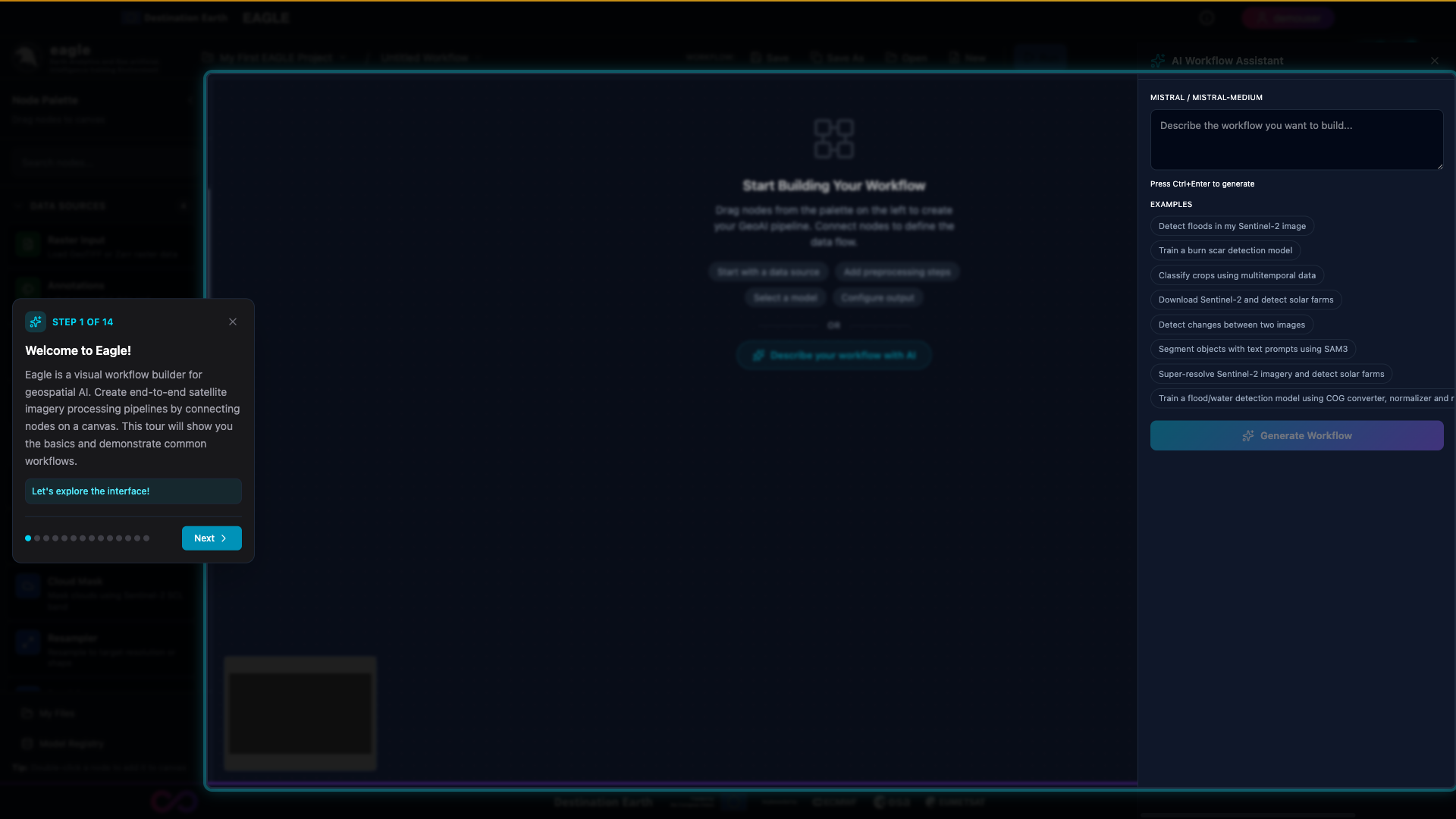
9.3. AI Workflow Assistant 

The AI Workflow Assistant generates complete workflows from natural-language descriptions and helps recover from execution errors.

Opening the Assistant: click the sparkle button in the bottom-right corner of the canvas. It only appears when the LLM service is configured and available.

Generating a workflow:

Type a description (e.g. “Detect floods in my Sentinel-2 image”).
Click Generate or press Enter.
Preview the generated workflow in the panel.
Click Apply to Canvas to load it.

Context-aware generation: when data-source nodes are already on the canvas with uploaded files, the assistant includes their metadata (band names, CRS, resolution, sensor type) in the prompt. If band names are generic (Band_1, …), it adds a Band Selector automatically; if the sensor is known, it selects compatible models. An indicator shows “Using metadata from N data source(s) on canvas”.

Fix with AI (error recovery): when a workflow fails, the error notification includes a Fix with AI button. Two strategies are used:

Deterministic fixes (pattern matching, no LLM call):
- “Need either masks or annotations” – replaces the Raster Input with a Training Dataset node that includes annotation masks.
- “Band mismatch / generic band names” – adds a Band Selector before the model.
- “Missing metrics node” – adds the required Metrics node.
LLM-based fixes – for other errors, the current workflow and the error message are sent to the LLM, which returns a corrected workflow.

What the assistant CAN fix (structural issues):

Wrong node connections (e.g. Raster Input connected directly to a training node instead of via Training Dataset).
Missing required nodes (no Annotations node, no Metrics node).
Wrong data source type for the task.
Band mismatches that need a Band Selector.
Incorrect workflow structure for a given task.

What the assistant CANNOT fix (it only sees the workflow graph and the error message):

Out-of-memory (OOM) errors – require reducing tile size, batch size, or choosing a smaller model.
Corrupted or missing data files – the AI cannot inspect or repair your GeoTIFF / Zarr files.
Data quality issues (wrong CRS, misaligned rasters, cloud-covered imagery, low resolution).
Model training failures (convergence, exploding gradients, wrong hyperparameters).
GPU / CUDA errors (driver issues, incompatible CUDA versions, hardware failures).
Inference on untrained models – if no checkpoint exists, the AI cannot create one.
Hyperparameter tuning (optimal learning rates, epochs, augmentation settings).
File-permission or disk-space issues.

Smart merge: when applying a generated or fixed workflow to a canvas that already has nodes, existing nodes are matched by ID first, then by type. Configured data (file paths, settings, uploaded files) is preserved on matched nodes; new nodes are added, missing nodes are removed, and positions are updated to the generated layout.

9.4. Model Registry 

The Model Registry tracks all fine-tuned models with versioning, lifecycle management, and comparison tools.

Opening the Registry: click the Model Registry button (database icon) at the bottom of the sidebar.

Tracked metadata (automatically recorded per training run): run name, task type, backbone, training config (epochs, batch size, learning rate, etc.), best metric (IoU, accuracy), final loss, checkpoint file path, creation and completion timestamps.

Model lifecycle:

completed – default after training finishes.
active – promoted as the go-to model for its task type (only one active per task).
archived – hidden from the default view but preserved in the database.
deprecated – marked as outdated.

Actions:

Promote (star icon) – make a model the active version for its task type. Assigns a version number and deactivates the previous active model.
Archive (box icon) – declutter the list.
Delete (trash icon) – permanently remove a model.
Rollback – in the detail view, revert to a previously active model.

Editing metadata: click any row to open the detail view and edit description, add comma-separated tags, or view the full training configuration.

Comparing models: select exactly two models with the checkboxes, click Compare – side-by-side config differences and overlaid loss curves are shown.

Filters: task type (flood-detection, burn-scars, etc.), status (completed / active / archived / deprecated), search by run name or description.

Using active models for inference: after promoting a model, inference nodes can automatically pick up the active model for their task type via the From Registry checkpoint option.

9.6. Interactive Tour 

Click the Tour button (play icon) in the header to start an in-product guided tour that covers project selection, canvas navigation, adding nodes, connecting nodes, running workflows, and viewing results. Highlighted areas show where to click, tooltips explain each feature, and a progress indicator tracks your position. You can restart the tour any time.

First step of the interactive tour — The first step of the interactive tour: a highlighted region with an inline tooltip and **Next / Skip** controls.

Tooltip shown after hovering over a node — Hovering over a node surfaces a contextual tooltip with a short description and the node’s expected inputs / outputs.

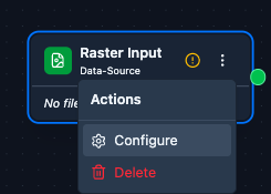
Three-dot context menu on a node — The three-dot menu on each node exposes per-node actions (duplicate, delete, view config JSON, etc.).

Inline warning shown on a node with an invalid configuration — Nodes with invalid configuration display an inline warning; clicking it opens an explanation of what needs to be fixed.

State after dismissing the warning — After acknowledging or fixing the warning, the indicator clears and the node returns to its normal state.

10. API Reference 

Eagle exposes a comprehensive REST API. The interactive Swagger UI is accessible at /docs on the service URL (e.g. https://eagle.destine.eu/docs). The OpenAPI specification itself is available at /api/openapi.

Key API endpoint groups:

Endpoint	Description
`/health`	Health check for Kubernetes probes (includes DB connectivity)
`/health/gpu`	GPU state and queue status
`/api/jobs`	Submit, monitor, and cancel workflow jobs
`/api/operations`	Query execution history and per-node status
`/api/workflows`	Save, load, list, and delete workflow definitions
`/api/projects`	Create, list, update, and delete projects
`/api/uploads`	Upload GeoTIFF, Zarr, and NetCDF files
`/api/fs`	Browse the project filesystem
`/api/sentinel2`	Search and download Sentinel-2 scenes
`/api/sam3`	Interactive SAM3 segmentation sessions
`/api/spectral`	Compute spectral profiles and indices
`/api/zonal`	Compute zonal statistics
`/api/geotiff`	Serve GeoTIFF tiles and previews
`/api/tiles`	Tile server for map previews
`/api/clip`	Clip rasters to AOIs
`/api/llm`	LLM-assisted workflow generation (“Fix with AI”)
`/api/advisor`	Data Advisor compatibility and quality analysis
`/api/registry`	Model Registry management
`/api/visualizations`	Visualization data endpoints
`/api/annotations`	Annotation projects and labels
`/api/share`	Workflow share links
`/api/downloads`	Package and download result files

For the full OpenAPI specification, see the API Documentation section.

11. Support and Contact 

For any technical issues, questions regarding analysis results, or to provide feedback on the Eagle service, please refer to the Support page.

Complete the contact form with all relevant details, and a member of the Destination Earth support team will provide assistance.