Showcasing the Climate DT in Action

The Climate DT produces globally consistent climate information at kilometre-scale resolution that enables analysis at local to regional scales. This page illustrates how the system can be used in practice, from global scale to European zooms and event-level case studies, giving examples of the added value of high-resolution coupled modelling.

Global and Regional Climate

The three Climate DT models (ICON, IFS-FESOM, IFS-NEMO) provide comprehensive global coverage at kilometre-scale resolutions (5 to 10 km), enabling climate analysis from global patterns to local features.

Globally consistent climate information with local granularity

The three Climate DT models are used for the production of Earth system information at 5 km global resolution, at scales where climate change impacts are observed and adaptation decisions are made, by harnessing Europe’s HPC systems, as shown in the figure below.

Global overlay of different variables from the three Climate DT model systems: ICON (left), IFS-FESOM (centre), and IFS-NEMO (right). The example snapshots show information from the atmosphere (clouds in white, precipitation rate in colours), and from the coupled ocean (temperature in colour, current speed via differences in brightness). Credit: ECMWF.

Zoom in on Europe: maximum precipitation

When zooming in, the Climate DT models provide a strong increase in local granularity compared to CMIP6, providing global information at a scale of previous regional information systems like the CERRA reanalysis and downscaled CORDEX simulations, as shown in the figure below.

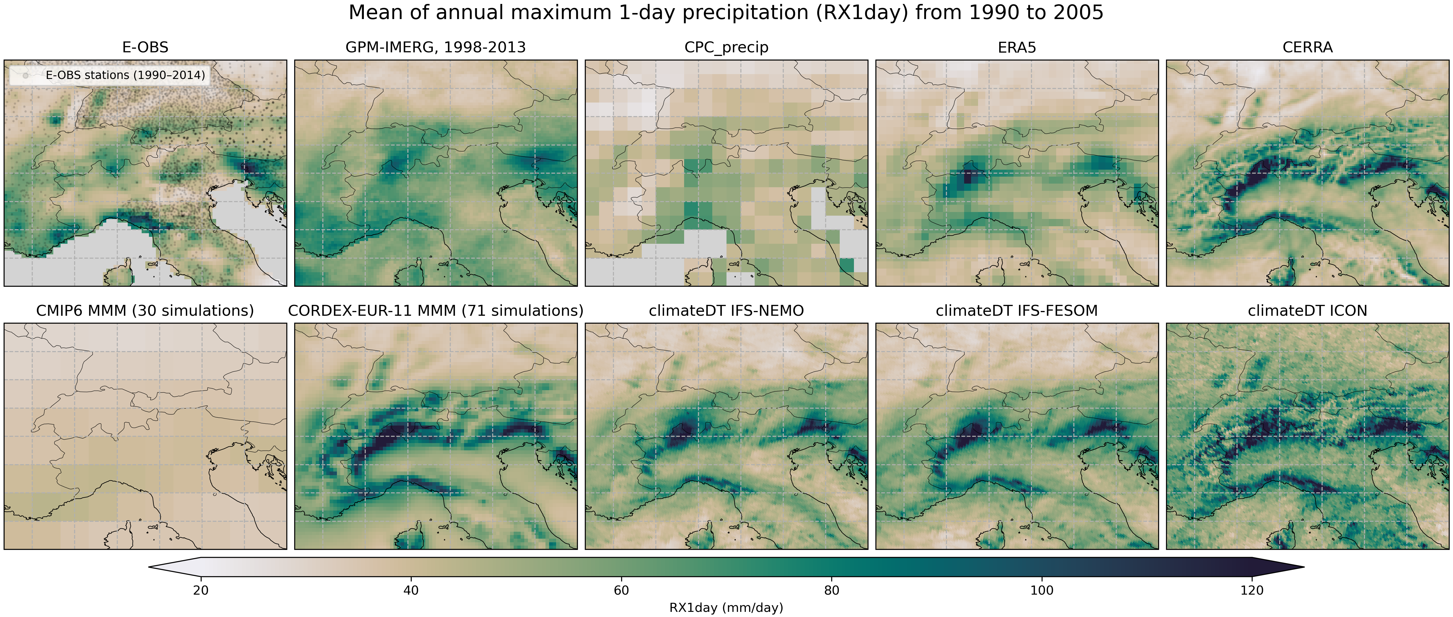
Mean of annual maximum 1-day precipitation (RX1day) from 1990 to 2005 from the Climate DT models (IFS-NEMO, IFS-FESOM and ICON), compared to the observational products E-OBS, GPM-IMERG and CPC, the reanalyses ERA5 and CERRA, produced by the Copernicus Climate Change Service (C3S), and the climate model ensembles CMIP6 and CORDEX-EUR-11. Credit: ECMWF

For the Climate DT models, the annual maximum of daily mean precipitation is computed for each year between 1990 and 2005 and averaged, using model output on the “high” resolution Healpix grid (“H1024”, ~6.4 km resolution). For the remaining datasets, RX1day is retrieved from the CDS Atlas and displayed on their respective grids.

Zoom in on Europe: maximum temperature

Similarly, for the Climate DT models, the annual maximum of hourly 2m temperature (TXX) is computed for each year between 1990 and 2005 and averaged. For the remaining datasets, TXX is again retrieved from the CDS Atlas and displayed on their respective grids. The Climate DT models capture the spatial patterns and magnitudes of TXX across Europe, with finer local details and sharper gradients than the coarser CMIP6 and CORDEX ensembles, while showing good agreement with the observational product E-OBS and the C3S reanalyses ERA5 and CERRA, as shown in the figure below.

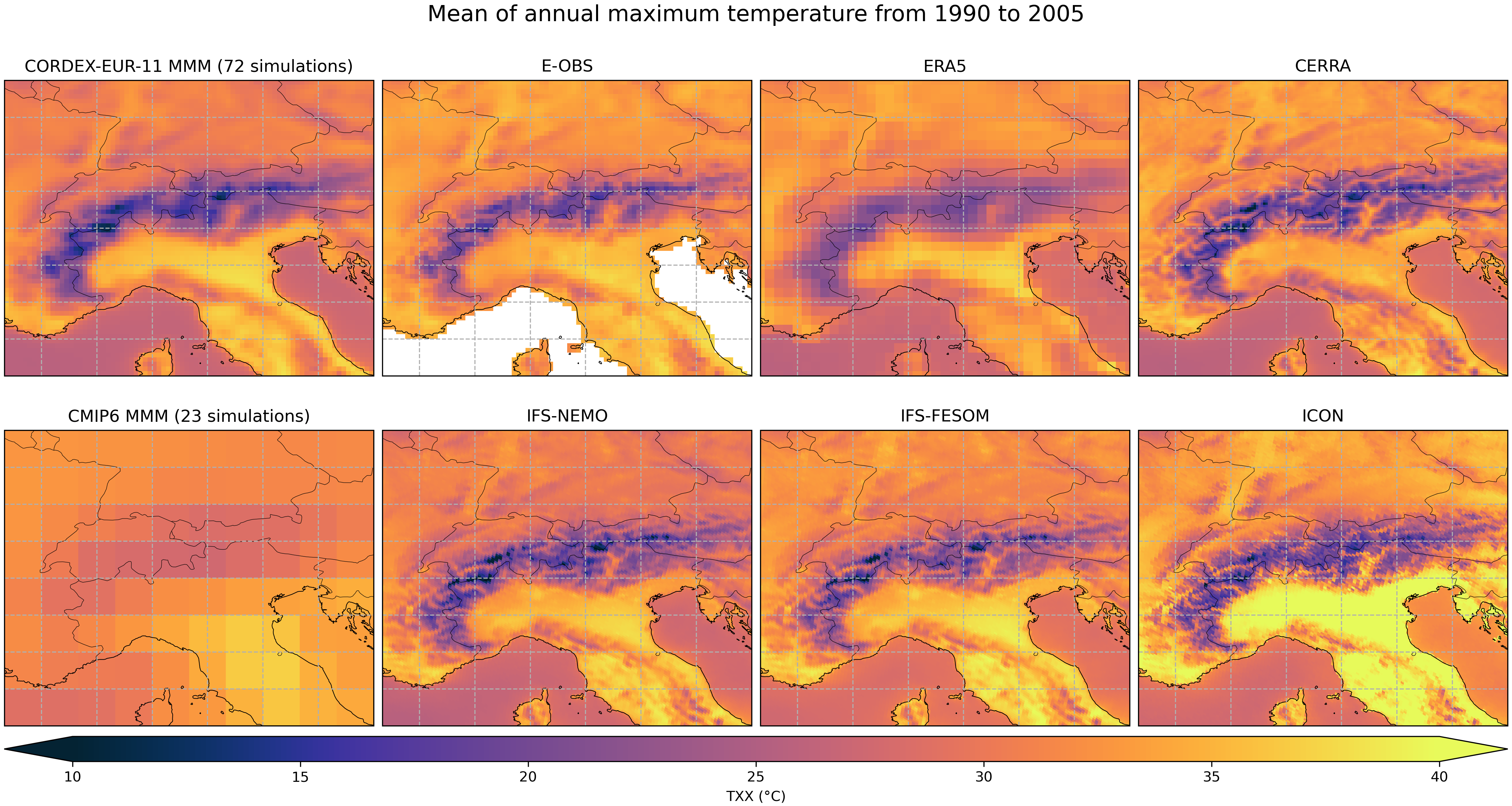
Mean of annual maximum temperature (TXX) from 1990 to 2005 from the Climate DT models (IFS-NEMO, IFS-FESOM and ICON), compared to the observational product E-OBS, the reanalyses ERA5 and CERRA and the climate model ensembles CMIP6 and CORDEX-EUR-11. Credit: ECMWF

Small Islands

The kilometre-scale resolution of the Climate DT enables explicit representation of small islands that are often poorly resolved or entirely missing in coarser global climate models, as shown in the figure below.

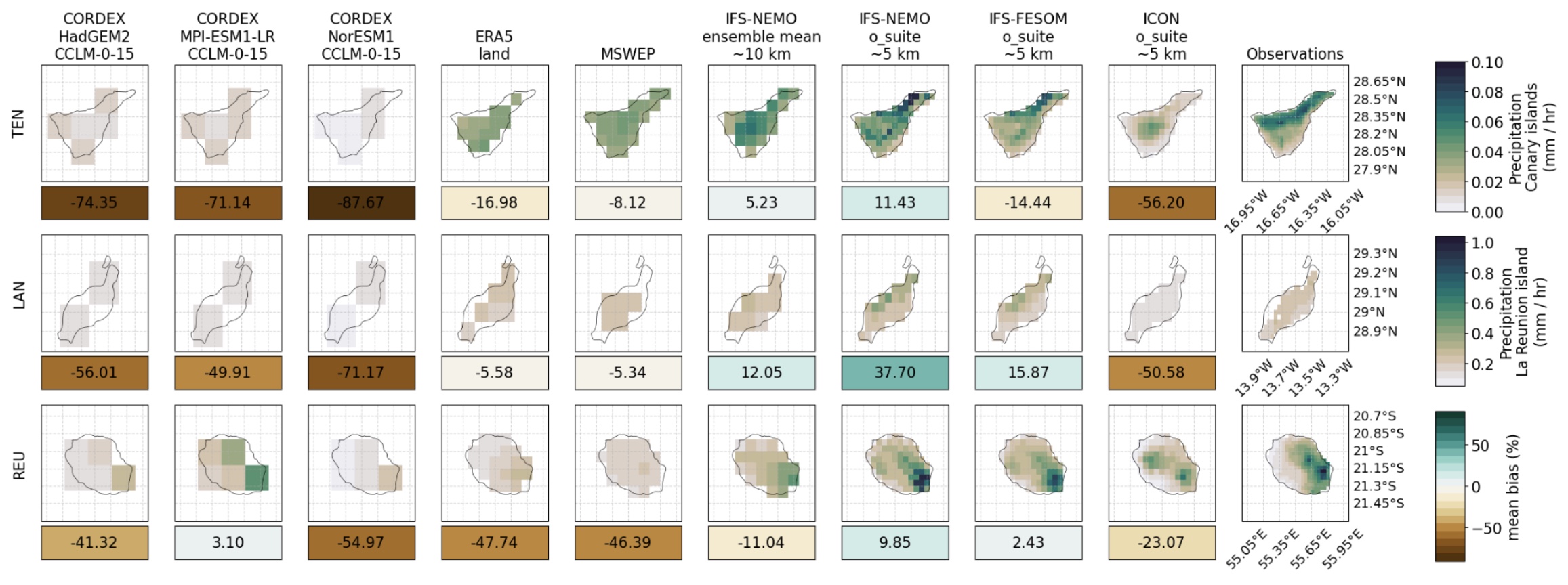
High-resolution representation of the islands of Tenerife (TEN), Lanzarote (LAN), and Réunion (REU) from the three Climate DT models. Maps show the average daily mean precipitation over the historical 1990-2014 period. Three CORDEX CORE models using the CCLM regional model and two reanalysis products (ERA5-land and MSWEP) are included for comparison. The heat maps below the maps show the mean bias for all models / reanalysis products compared to the gridded observations provided by Agencia Estatal de Meteorología (AEMET) (TEN and LAN) and Météo-France (REU). The mean bias is calculated by interpolating (using the conservative_normed interpolation method with land / sea mask included) the observations on the model / reanalysis grid then taking the average difference between the model and observations. Values given as a percentage of the observational values. Credit: BSC.

Urban Heat Islands

The Climate DT models can capture many aspects of km-scale surface phenomena. In particular, the km-scale resolution can also capture the spatial structure of urban heat islands with fidelity comparable to satellite observations. As an example, the figure below shows the modelled Berlin urban heat island, compared to observed land surface temperature.

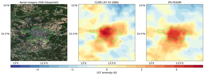
Left: aerial imagery of Berlin and surroundings for reference. Centre: observed land surface temperature (LST) version 2 and EUMETSAT LSA SAF Land Surface Temperature (MLST). Right: modelled LST from IFS-FESOM. Both observed and modelled LST show the spatial anomaly of mean values at 14 UTC (12 pm local time) for the 2018–2022 JJA period, after filtering out cloudy pixels (cloud cover > 0.3). The green dashed contour shows the urban cluster for Berlin, following Pedruzo-Bagazgoitia et al. (2026).

Storyline Examples

Within the Climate DT, storyline simulations are designed to replay weather events under different climate states: past (~1950 conditions), present-day, and a future scenario with +2K warming. Here, the storyline simulation approach is demonstrated through two high-impact European extreme events, Storm Boris (September 2024), and the Paris heatwave (July 2019). For both cases further details are presented by John et al. (2026).

Importantly, while two events are highlighted here, the storyline simulations can be used to assess how any extreme event that occurred between 2017 and 2025 could evolve in different climate conditions.

Storm Boris (September 2024)

Maps of 5-day accumulated precipitation for Storm Boris (below) compare the km-scale IFS-FESOM ensemble against a coarser climate model run (based on the CMIP6 model AWI-CM1), and to reference reanalysis and observational datasets (ERA5, MSWEP). The present-day IFS-FESOM ensemble accurately reproduces the spatial structure and magnitude of the observed extreme precipitation, demonstrating the added value of km-scale resolution over coarser models. The three-scenario comparison — past, present-day, and future +2K — reveals how the thermodynamic response to warming amplifies precipitation in this event.

5-day accumulated precipitation (mm) for Storm Boris (12–16 September 2024). Top row: (a) AWI-CM1 coarse-resolution nudged run, (b) ERA5 reanalysis, (c) MSWEP observations. Bottom row: ensemble mean from nudged km-scale IFS-FESOM storyline experiments for (d) past climate, (e) present-day climate, (f) future +2K climate.

Paris Heatwave (25 July 2019)

Maximum 2m-temperature during the peak of the 25 July 2019 European heatwave (below) shows that the historical IFS-FESOM ensemble faithfully captures the spatial gradients and peak magnitudes of the observed event compared to ERA5 and E-OBS. The km-scale resolution resolves fine-scale temperature contrasts — including urban heat island signatures and orographic effects — that are smoothed out in the coarser AWI-CM1 run and ERA5. Under the +2K future scenario, the area exceeding 40 °C expands substantially, extending from France and Iberia into Germany and the Benelux region, while the past scenario shows peak temperatures remaining below 35 °C over much of France. Simulating this event for the three climate states assesses the regional intensification of the heatwave.

Maximum 2m-temperature (°C) during the peak of the 25 July 2019 European heatwave. Top row: (a) AWI-CM1 coarse-resolution nudged run, (b) ERA5 reanalysis, (c) E-OBS observations. Bottom row: ensemble mean from nudged km-scale IFS-FESOM storyline experiments for (d) past climate, (e) present-day climate, (f) future +2K climate.